Sample rate and bit depth are technical parameters in digital audio processing. The sample rate is the number of samples taken per second to represent a continuous audio signal, while the bit depth is the number of bits used to represent each sample’s amplitude. These parameters significantly impact the accuracy and quality of the digital audio output.

Standards Used In Audio Processing:

Sample Rate:

44.1 kHz, 48 kHz, 88.2 kHz, 96 kHz, and 192 kHz. 44.1 kHz is the most commonly used sample rate, and is the standard for CD-quality audio. Higher sample rates are used in high-resolution audio and for certain applications like film and video production.

Bit Depth:

16-bit, 24-bit, and 32-bit. 16-bit is the standard for CD-quality (and mp3) audio and is commonly used for streaming and other digital audio applications. 24-bit and 32-bit (floating point) are used in high-resolution audio and for professional audio production and mastering.

This text explains the fundamental concepts of how analog sound is converted to digital format through the sampling process.

Sound Wave Basics:

• Sound waves are continuous signals
• They contain infinite signal values over time

Signal Conversion Process:

• Microphone captures sound waves and converts them to electrical signals
• Analog-to-Digital Converter (ADC) converts electrical signals to digital format

Sampling Concept:

• Definition: Measuring continuous signal values at fixed time intervals
• Result: Creates a discrete waveform with finite values at uniform intervals

Sampling Rate:

• Measured in Hertz (Hz)
• Represents number of samples per second
• Example: CD-quality audio uses 44,100 Hz (44,100 samples per second)

Amplitude

The text explains how amplitude relates to sound pressure and provides real-world examples to illustrate different sound intensity levels.

Amplitude Definition:

• Represents sound pressure level at any moment
• Measured in decibels (dB)
• Results from changes in air pressure at audible frequencies

Human Perception:

• Amplitude is perceived as loudness
• Examples of sound levels:
  • Normal speaking voice: < 60 dB
  • Rock concert: ~125 dB (near human hearing limits)

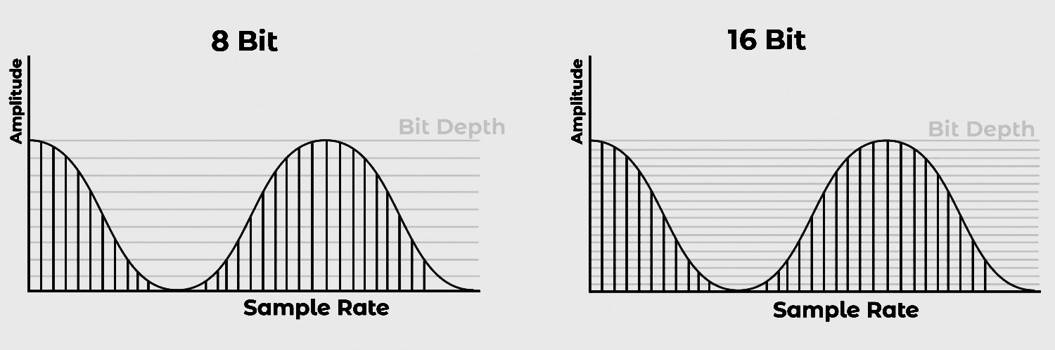
Bit depth

Bit depth determines the number of possible discrete amplitude values we can utilize for each audio sample. The higher the bit depth, the more amplitude values are available per sample

Bit Depth Basics:

• Determines precision of amplitude measurement in audio samples
• Higher bit depth = better approximation of original sound wave

Common Bit Depths:

• 16-bit: 65,536 possible amplitude steps
• 24-bit: 16,777,216 possible amplitude steps

32-bit Audio:

• Uses floating-point values (unlike 16/24-bit which use integers)
• Actual precision equals 24-bit depth
• Values range between -1.0 and 1.0
• Preferred for machine learning models
• Requires conversion to floating-point format for model training

Quick reference: key concepts

Sample — One measurement of the audio signal at one instant in time. The sample rate (e.g. 16 000 Hz) is how many samples we take per second.

Amplitude — The “height” of the waveform at a given moment: how far the signal is from zero. In the array, each number is the amplitude at that time step. We hear it as loudness (bigger absolute value ≈ louder).

The array — A 1D list of numbers: index = time (e.g. index 0 → t=0, index 1 → t=1/sample_rate), value = amplitude at that time. So we have (time, amplitude) pairs — one amplitude per sample.

Pitch — How high or low a sound is; we perceive it from frequency (how many times the wave repeats per second, in Hz). Pitch is not stored directly in the array. It comes from the pattern of amplitudes over time (e.g. via FFT/spectrum).

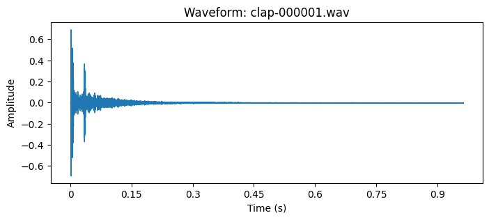
Waveform Visualization

This section demonstrates the visualization of audio waveforms using matplotlib and librosa. The waveform representation plots the amplitude of the audio signal as a function of time, providing a temporal visualization of the sound's pressure variations. The resulting plot features amplitude measurements on the vertical axis and temporal progression on the horizontal axis, enabling detailed analysis of the audio signal's characteristics.

Python modules

This project requires the following python modules:

import os
import librosa
import librosa.display
import matplotlib.pyplot as plt
import IPython.display as ipd
import numpy as np
import torch
import torchaudio

Print audio file of a clap

file = 'clap-000001.wav'
array, sampling_rate = librosa.load(os.path.join('my-path', file))
print(array, sampling_rate)

<audio controls> <source src="../public/assets/airasoul/clap-000001.wav" type="audio/wav"> Your browser does not support the audio element. </audio>

Print waveform

file = 'clap-000001.wav'
array, sampling_rate = librosa.load(os.path.join('my-path', file))

plt.figure(figsize=(8, 3))
librosa.display.waveshow(array, sr=sampling_rate)
plt.title(f'Waveform: {file}')
plt.xlabel('Time (s)')
plt.ylabel('Amplitude')
ipd.display(ipd.Audio(array, rate=sampling_rate))
plt.show()

Loading an Audio file

When you load a WAV with librosa.load(), you get a 1D array of floats — one number per sample. Below we load a short clip and print the array’s shape, dtype, and the first 20 sample values so you can see exactly what the model (or any code) receives.

Load one short file

array, sr = librosa.load(os.path.join("drum-kit/data/clap", "clap-000001.wav"))

print("Shape (number of samples):", array.shape)
print("Dtype:", array.dtype)
print("First 20 sample values:")
print(array[:20])
print("...")
print("Last 5 values:", array[-5:])
print("Min:", array.min(), "| Max:", array.max())

Output

Shape (number of samples): (21237,)
Dtype: float32
First 20 sample values:
[ 0.00752919  0.0012277  -0.00382459 -0.00844482  0.00743008  0.05842568
  0.01708915 -0.07676509  0.09604676  0.31853813  0.01520596 -0.39263156
 -0.19292395  0.02274308 -0.29928595 -0.30348873  0.37696874  0.6934469
  0.24533717 -0.16166289]
...
Last 5 values: [-3.2663316e-05 -1.1256659e-04 -3.0112578e-04 -4.5693252e-04
 -2.6061770e-04]
Min: -0.5205457 | Max: 0.6934469

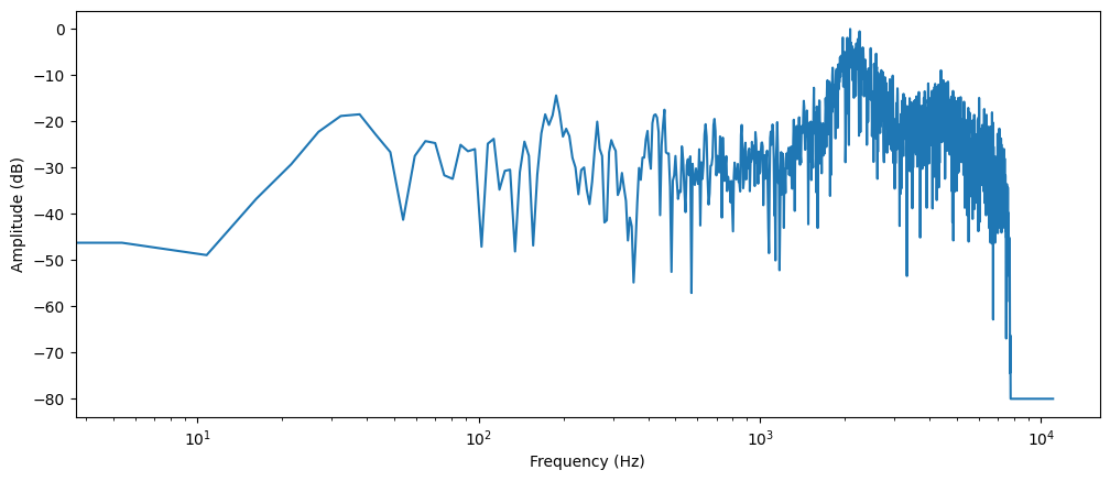
The frequency spectrum

The frequency spectrum analysis provides an alternative method for audio signal visualization, commonly referred to as the frequency domain representation. This representation is obtained through the application of the Discrete Fourier Transform (DFT), a mathematical technique that decomposes a signal into its constituent frequency components. The resulting spectrum reveals both the frequency distribution and the corresponding magnitude of each component within the signal.

To visualize the frequency components of a clap sound, we'll compute its DFT using NumPy's rfft() function. Although the DFT can be applied to the entire audio signal, analyzing a shorter segment provides more meaningful insights. For this demonstration, we'll focus on the first 4096 samples, which captures the initial impact of the clap:

# Print frequency spectrum
array, sampling_rate = librosa.load(os.path.join('drum-kit/data/clap/clap-000001.wav'))

# take the first 4096 samples
dft_input = array[:4096]

# calculate the DFT
window = np.hanning(len(dft_input))
windowed_input = dft_input * window
dft = np.fft.rfft(windowed_input)

# get the amplitude spectrum in decibels
amplitude = np.abs(dft)
amplitude_db = librosa.amplitude_to_db(amplitude, ref=np.max)

# get the frequency bins
frequency = librosa.fft_frequencies(sr=sampling_rate, n_fft=len(dft_input))

plt.figure().set_figwidth(12)
plt.plot(frequency, amplitude_db)
plt.xlabel("Frequency (Hz)")
plt.ylabel("Amplitude (dB)")
plt.xscale("log")
plt.show()

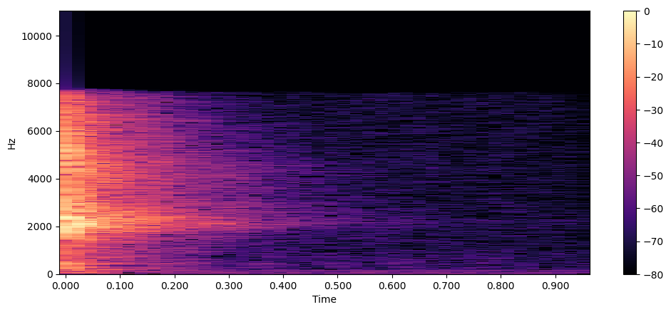
Spectrogram Analysis

The spectrogram provides a comprehensive three-dimensional representation of audio signals, displaying frequency content evolution over time. While a standard frequency spectrum offers only a momentary snapshot, the spectrogram reveals the dynamic nature of frequency components through time-frequency analysis.

The Short-Time Fourier Transform (STFT) algorithm generates spectrograms by computing successive Discrete Fourier Transforms (DFTs) across small, overlapping time windows. This process yields a time-frequency representation where:

• X-axis: Temporal progression
• Y-axis: Frequency (Hz)
• Color intensity: Amplitude/power in decibels (dB)
• High intensity (bright) = dominant frequencies in the audio
  • Low intensity (dark) = minimal or background frequencies
  • Color variations show how loud different frequencies are at each moment

Using librosa's STFT implementation, we analyze audio signals with a default window size of 2048 samples, optimizing the balance between temporal and frequency resolution. This configuration enables detailed visualization of frequency components while maintaining temporal precision.

Let's generate a spectrogram using librosa's stft() and specshow() functions:

array, sampling_rate = librosa.load(os.path.join('drum-kit/data/clap/clap-000001.wav'))

D = librosa.stft(array)
S_db = librosa.amplitude_to_db(np.abs(D), ref=np.max)

plt.figure().set_figwidth(12)
librosa.display.specshow(S_db, x_axis="time", y_axis="hz")
plt.colorbar()

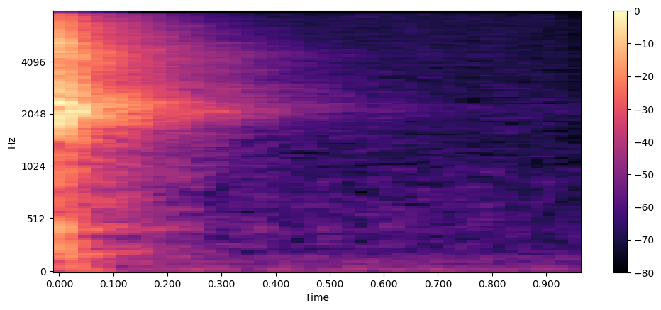
Mel Spectrogram Analysis

The mel spectrogram represents a perceptually-aligned variation of the standard spectrogram, optimized for speech processing and machine learning applications. While retaining temporal-frequency relationships, it incorporates the mel scale—a psychoacoustic frequency mapping that mirrors human auditory perception.

The process involves two key steps:

1. Short-Time Fourier Transform (STFT) computation
2. Mel filterbank application for frequency warping

This transformation accounts for the human ear's logarithmic sensitivity to frequency changes, providing enhanced resolution in lower frequencies where human hearing is most discriminative.

Implementation using librosa's melspectrogram() function:

array, sampling_rate = librosa.load(os.path.join('drum-kit/data/clap/clap-000001.wav'))

S = librosa.feature.melspectrogram(y=array, sr=sampling_rate, n_mels=128, fmax=8000)
S_dB = librosa.power_to_db(S, ref=np.max)

plt.figure().set_figwidth(12)
librosa.display.specshow(S_dB, x_axis="time", y_axis="mel", sr=sampling_rate, fmax=8000)
plt.colorbar()

Conclusion

Digital audio is a chain of choices: sample rate and bit depth at capture, then a 1D array of amplitudes in code — one float per instant in time. That array is what librosa.load() gives you, and it is the starting point for almost everything else in this post.

We looked at the same audio clip three ways. A waveform shows loudness over time. A frequency spectrum (DFT on a short window) shows which frequencies are present at one moment. A spectrogram (STFT) stacks those snapshots so you can see how energy moves across frequency and time. A mel spectrogram warps frequency to match human hearing.